이 실습 노트에서는 글로벌 기상 및 대기질 데이터인 openweather.parquet 데이터를 활용하여 pandas의 핵심 기능인 그룹화와 집계(Split-Apply-Combine) 연산 패턴을 단계별로 수행합니다. 해당 데이터셋에는 국가 및 도시별 대기오염 물질(PM2.5, PM10 등) 농도와 기상 정보(기온, 습도, 풍속 등)가 포함되어 있어 다차원 집계 연산을 연습하기에 적합합니다.
본 실습에서는 단순 집계부터 구간화(Binning), 다중 집계(agg), 형태 보존 변환(transform), 그룹 필터링(filter), 그리고 정교한 그룹별 사용자 정의 연산(apply)까지 다루며, 각 단계의 집계 결과를 직관적으로 이해할 수 있는 시각화 차트를 함께 구현합니다.
13.1 데이터 로드 및 초기 탐색
필요한 라이브러리를 불러오고, 운영체제별 한글 폰트를 설정한 후 대기질 데이터를 PyArrow 백엔드(engine="pyarrow", dtype_backend="pyarrow")로 로드합니다.
import platformimport pandas as pdimport numpy as npimport matplotlib.pyplot as pltimport seaborn as sns# 운영체제별 한글 폰트 설정if platform.system() =="Darwin": plt.rcParams["font.family"] ="Apple SD Gothic Neo"elif platform.system() =="Windows": plt.rcParams["font.family"] ="Malgun Gothic"else: plt.rcParams["font.family"] ="NanumGothic"plt.rcParams["axes.unicode_minus"] =False# 대기질 데이터 로드 (PyArrow 백엔드 지정)df = pd.read_parquet("../data/openweather.parquet", engine="pyarrow", dtype_backend="pyarrow",)# 데이터 구조 및 기본 정보 확인print(f"데이터 전체 크기: {df.shape}")print( df[ ["continent","country_name","city_name","temp","humidity","pm2_5", ] ].head(3))
데이터 전체 크기: (64667, 88)
  continent          country_name  ... humidity  pm2_5
0        EU               Andorra  ...       75   4.71
1        EU               Andorra  ...       75   4.71
2        AS  United Arab Emirates  ...       24  28.41

[3 rows x 6 columns]
13.2 기본적인 GroupBy 사용법 및 인덱스 제어
데이터를 특정 기준에 따라 분할(Split)하고 단순 통계량을 집계(Apply & Combine)하는 기본 사용법과, 집계 결과의 인덱스 형태를 제어하는 as_index 매개변수를 비교 학습합니다.
13.2.1 단일 및 다중 컬럼 기준 그룹화
국가(country_name)별로 데이터를 그룹화하여 미세먼지(pm2_5) 농도의 평균을 산출합니다. 기본적으로 그룹화 키는 결과 시리즈의 인덱스로 지정됩니다.
# 국가별 PM2.5 평균 계산 (기본값 as_index=True)country_pm25 = df.groupby("country_name")["pm2_5"].mean()print(country_pm25.head(5))
groupby() 연산 후 인덱스를 보존해야 하는 정밀한 라벨링 분석에서는 as_index=True(기본값)를 사용하고, 시각화 라이브러리(Seaborn 등)나 Tidy Data 포맷으로 연계할 때는 as_index=False 또는 연산 후 .reset_index()를 연결하여 사용하는 것이 깔끔합니다.
13.3 연속형 변수 구간화(Binning) 기반 그룹화
연속형 숫자 데이터를 pd.cut() 함수로 명확한 범주형 구간(Bins)으로 변환한 뒤, 해당 범주를 기준으로 그룹화 연산을 수행할 수 있습니다.
여기서는 PM2.5 농도를 기준으로 세계보건기구(WHO) 및 대기질 지수 기준에 맞추어 4단계 등급(Air_Quality: ‘Good’, ‘Moderate’, ‘Unhealthy’, ‘Very Unhealthy’)으로 분류하고, 등급별 기온, 습도, 풍속의 평균을 비교합니다.
# PM2.5 농도를 기준으로 대기질 구간 생성bins = [0, 15, 35, 75, float("inf")]labels = ["Good", "Moderate", "Unhealthy", "Very Unhealthy"]df["Air_Quality"] = pd.cut( df["pm2_5"], bins=bins, labels=labels)# 대기질 등급별 주요 기상 요인 평균 집계 (observed=False 지정)quality_summary = df.groupby("Air_Quality", observed=False)[ ["temp", "humidity", "wind_speed"]].mean()print(quality_summary)
pandas 최신 버전에서는 범주형(Categorical) 변수를 기준으로 그룹화할 때 observed=False를 명시하여 관측되지 않은 범주 조합까지 모두 포함할지 여부를 제어합니다. 명시적으로 지정해 줌으로써 수식 경고(FutureWarning)를 방지하고 예견된 집계 결과를 얻을 수 있습니다.
13.4 다중 집계와 시각화 (agg 메서드 활용)
agg() 메서드는 하나 이상의 집계 함수를 여러 컬럼에 동시에 다르게 적용할 수 있어 다각도의 요약 통계량을 생성할 때 강력합니다.
13.4.1 국가별 대기질 요약 및 시각화
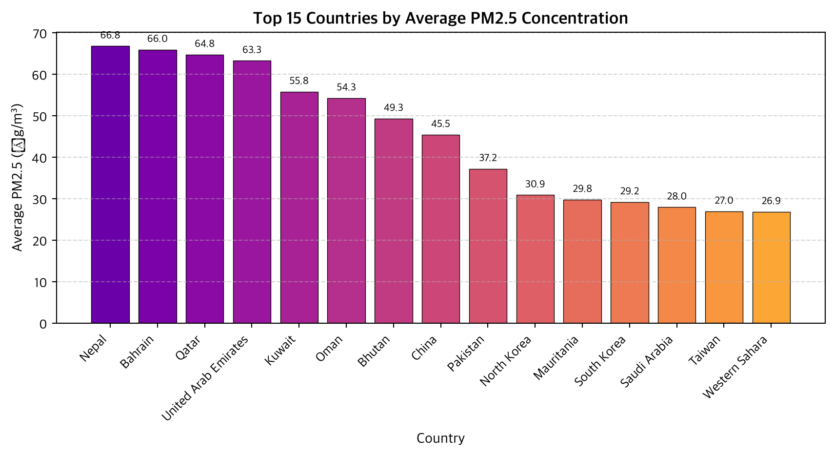
국가별로 미세먼지(pm2_5)의 평균(mean), 최댓값(max), 표준편차(std)를 동시에 산출하고, 평균 PM2.5 농도가 가장 높은 상위 15개 국가를 시각화합니다.
# 국가별 PM2.5 요약 통계량 산출 (agg 활용)pm25_summary = df.groupby('country_name')['pm2_5'].agg( mean_pm25='mean', max_pm25='max', std_pm25='std').reset_index()# 평균 PM2.5 농도 상위 15개국 추출top15_pm25 = pm25_summary.sort_values(by='mean_pm25', ascending=False).head(15)# 상위 15개국 출력print(top15_pm25.head(5))# 시각화plt.figure(figsize=(9, 5))colors = plt.cm.plasma(np.linspace(0.2, 0.8, len(top15_pm25)))bars = plt.bar(top15_pm25['country_name'], top15_pm25['mean_pm25'], color=colors, edgecolor='black', linewidth=0.5)plt.title('Top 15 Countries by Average PM2.5 Concentration', fontsize=13, fontweight='bold')plt.xlabel('Country', fontsize=11)plt.ylabel('Average PM2.5 (µg/m³)', fontsize=11)plt.xticks(rotation=45, ha='right')plt.grid(axis='y', linestyle='--', alpha=0.5)# 수치 라벨 추가for bar in bars: height = bar.get_height() plt.text(bar.get_x() + bar.get_width()/2., height +1,f'{height:.1f}', ha='center', va='bottom', fontsize=8)plt.tight_layout()plt.show()
groupby().transform() 연산은 그룹별 집계 결과를 축약(Collapse)하지 않고, 원본 데이터프레임과 동일한 길이의 인덱스 형태를 유지한 채 각 관측치 위치에 집계값을 1:1로 매핑하여 반환합니다.
이 특성을 활용하면 “개별 관측 도시의 PM2.5 농도가 해당 국가 전체 평균 대비 얼마나 치우쳐 있는지”의 편차(Deviation)를 손쉽게 산출할 수 있습니다.
13.5.1 국가 대비 편차 계산 및 분포 시각화
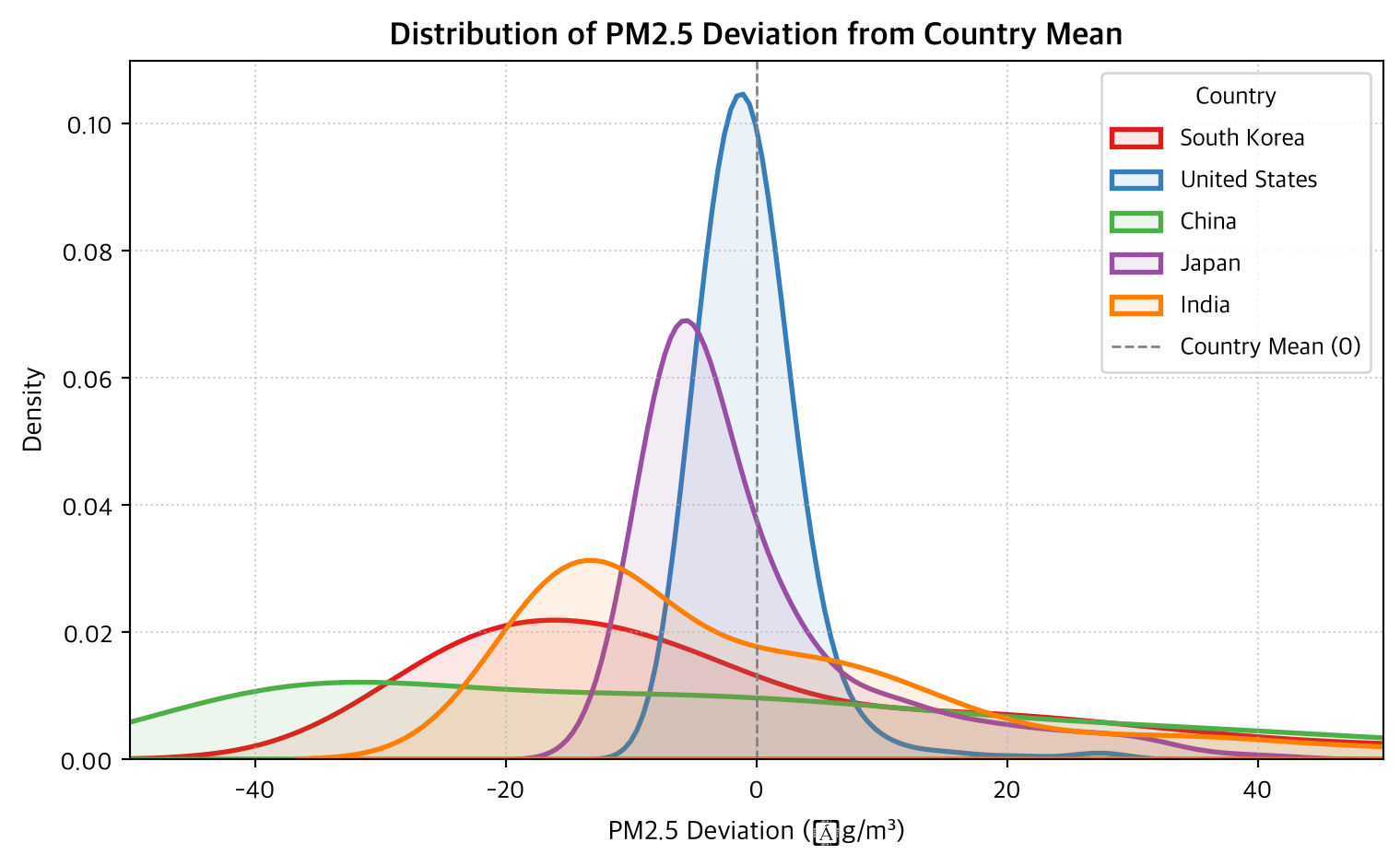
각 관측 데이터의 PM2.5 농도에서 소속 국가의 평균 PM2.5 농도를 뺀 편차(PM2.5_Deviation)를 계산하고, 대표적인 5개 국가(South Korea, United States, China, Japan, India)의 편차 분포를 커널 밀도 추정(KDE) 곡선으로 비교 시각화합니다.
# transform을 이용해 국가별 평균을 원본 데이터 행 크기로 확장df["Country_Mean_PM2.5"] = df.groupby("country_name")["pm2_5"].transform("mean")# 국가 평균 대비 개별 관측값의 편차 계산df["PM2.5_Deviation"] = ( df["pm2_5"] - df["Country_Mean_PM2.5"])# 대상 국가 선택target_countries = ["South Korea","United States","China","Japan","India",]df_selected = df[ df["country_name"].isin(target_countries)].copy()# 시각화plt.figure(figsize=(8, 5))palette = ["#e41a1c","#377eb8","#4daf4a","#984ea3","#ff7f00",]for idx, country inenumerate(target_countries): country_data = df_selected[ df_selected["country_name"] == country ]ifnot country_data.empty: sns.kdeplot( data=country_data["PM2.5_Deviation"], label=country, color=palette[idx], linewidth=2, fill=True, alpha=0.1, )plt.title("Distribution of PM2.5 Deviation from Country Mean", fontsize=13, fontweight="bold",)plt.xlabel("PM2.5 Deviation (µg/m³)", fontsize=11)plt.ylabel("Density", fontsize=11)plt.axvline(0, color="gray", linestyle="--", linewidth=1, label="Country Mean (0)",)plt.legend(title="Country", frameon=True)plt.xlim(-50, 50)plt.grid(True, linestyle=":", alpha=0.6)plt.tight_layout()plt.show()
그림 13.2: 주요 국가별 국가 평균 대비 PM2.5 편차 분포(KDE).
agg나 mean 연산은 데이터 행 수가 그룹 수만큼 줄어드는 축약 연산인 반면, transform은 원본 데이터프레임에 그룹 통계량 열을 직접 추가하거나(Column augmentation) 정규화, 편차 산출 등 1:1 대치 연산 시 필수적으로 쓰입니다.
13.6 조건 기반 그룹 선택 (filter 메서드 활용)
groupby().filter() 메서드는 그룹 단위로 boolean 조건을 적용하여 조건이 참(True)인 그룹 전체의 행 데이터를 필터링하여 반환합니다. 개별 행 필터링인 df.query()나 df[...]와 구분되는 개념입니다.
여기서는 관측 데이터 수가 300건 이상이고, 동시에 국가 평균 PM2.5 농도가 25 µg/m³를 초과하는 “대기 오염 집중 관리 대상 국가 그룹”을 선별합니다.
# 그룹 단위 필터링 조건 적용 (데이터 수 >= 300건 & 평균 PM2.5 > 25)focused_df = df.groupby("country_name").filter(lambda x: (len(x) >=300) and (x["pm2_5"].mean() >25))print(focused_df["country_name"].unique())print(f"필터링된 전체 행 수: {focused_df.shape[0]} / 원본 전체 행 수: {df.shape[0]}")
pandas 2.2 이상에서는 groupby().apply() 연산 시 그룹화에 사용된 컬럼이 전달되는 함수 내부 데이터프레임에 유지되는 것에 대해 경고를 출력합니다. include_groups=False를 명시함으로써 그룹 키 컬럼과의 충돌 없는 명확한 서브 데이터프레임 연산을 보장합니다.