import platform
import pandas as pd
import pyarrow as pa
import pyarrow.compute as pc
import pyarrow.dataset as ds
import matplotlib.pyplot as plt
import seaborn as sns
from pathlib import Path

# 운영체제별 한글 폰트 설정
if platform.system() == "Darwin":
    plt.rcParams["font.family"] = "Apple SD Gothic Neo"
elif platform.system() == "Windows":
    plt.rcParams["font.family"] = "Malgun Gothic"
else:
    plt.rcParams["font.family"] = "NanumGothic"

plt.rcParams["axes.unicode_minus"] = False

# 데이터 디렉터리 경로 설정
data_dir = Path(
    "../data/instacart-market-basket-analysis-parquet"
)5 실습: PyArrow
Kaggle의
Instacart Market Basket Analysis데이터셋을 바탕으로 PyArrow을 활용해서 EDA 과정을 다시 한 번 실습을 진행해보겠습니다.
Kaggle의 Instacart Market Basket Analysis(이하 Instacart 데이터셋)은 유저들의 온라인 식료품 주문 내역(약 3,400만 건의 장바구니 상품 내역)을 포함하고 있습니다. 이번 실습에서는 instacart-market-basket-analysis-parquet 디렉터리에 저장된 Parquet 포맷의 데이터셋을 활용하여 아래 3가지 핵심 주제를 실습합니다.
- pandas에서 PyArrow 활용
- 주문 요일 및 시간대별 주문 분포와 재주문 간격 분석
- 장바구니 담긴 순서 및 카테고리별 재주문율 분석
필요한 라이브러리를 가져옵니다.
- pyarrow (
pa):pyarrow는 Apache Arrow 의 Python 바인딩으로, 메모리 내 열 기반 데이터 표현을 위한 라이브러리입니다. pandas 의 DataFrame 을 pyarrow.Table 로 변환하면, 대용량 데이터 처리 시 메모리 효율성과 성능을 크게 향상시킬 수 있습니다.- 열 기반: CPU 캐시 효율성을 높여 분석 성능을 극대화
- 영복사(zero-copy): pandas, NumPy, Spark 등 다른 시스템과 메모리 공유 가능
- 직렬화 포맷: Parquet, Feather 등
- pyarrow.compute (
pc):pyarrow.compute모듈은 Arrow 배열에 대한 벡터화된 연산 함수들을 제공합니다. 이 모듈을 사용하면 pandas 의 apply() 보다 훨씬 빠른 속도로 대용량 데이터를 처리할 수 있습니다.- 산술 연산:
pc.add(),pc.subtract(),pc.multiply()등 - 집계 함수:
pc.sum(),pc.mean(),pc.min(),pc.max()등 - 논리 연산 및 비교:
pc.equal(),pc.greater(),pc.is_null()등 - 문자열 및 날짜 처리:
pc.utf8_trim(),pc.year(),pc.month()등
- 산술 연산:
- pyarrow.dataset (
ds):pyarrow.dataset은 디스크나 클라우드 스토리지에 저장된 대용량 데이터셋을 효율적으로 조회하고 처리하기 위한 고수준 API를 제공합니다. 예를 들어,ds.dataset("data/", format="parquet").to_table(filter=ds.field("year") == 2025)를 사용하면 2025년 데이터만 필터링하여 읽을 수 있습니다.- 파티셔닝된 데이터셋:
ds.dataset("data/", format="parquet")과 같이 디렉터리 구조를 인식 - 필터링 및 열 선택: 필요한 데이터만 메모리에 로드하여 효율적인 처리
- 클라우드 스토리지 지원: S3, GCS 등 다양한 스토리지 지원
- 파티셔닝된 데이터셋:
- pathlib.Path:
pathlib은 파일 및 디렉터리 경로를 객체 지향적으로 다루기 위한 표준 라이브러리입니다. Path 클래스를 사용하면 운영체제에 독립적인 경로 연산이 가능합니다. 예를 들어,Path("data") / "file.parquet"는 운영체제에 맞게 해석됩니다.- OS 간 호환성: 윈도우 (
\) 와 유닉스 (/) 의 경로 구분자를 자동으로 처리 - 직관적인 메서드:
Path("data") / "file.parquet"와 같이 경로 연결이 가능 - 파일 시스템 작업:
exists(),mkdir(),glob()등 다양한 파일 시스템 작업을 제공
- OS 간 호환성: 윈도우 (
5.1 데이터 로드 및 PyArrow 백엔드 검증
pandas 3.x에서는 read_parquet() 호출 시 dtype_backend="pyarrow"를 지정하여 전통적인 NumPy 백엔드 대신 ArrowDtype을 기반으로 데이터를 저장할 수 있습니다. 먼저, orders, products, aisles, departments 메타데이터 테이블을 PyArrow 백엔드로 읽어옵니다.
orders = pd.read_parquet(
    data_dir / "orders.parquet",
    engine="pyarrow",
    dtype_backend="pyarrow",
)
products = pd.read_parquet(
    data_dir / "products.parquet",
    engine="pyarrow",
    dtype_backend="pyarrow",
)
aisles = pd.read_parquet(
    data_dir / "aisles.parquet",
    engine="pyarrow",
    dtype_backend="pyarrow",
)
departments = pd.read_parquet(
    data_dir / "departments.parquet",
    engine="pyarrow",
    dtype_backend="pyarrow",
)

# orders 데이터프레임의 스키마 및 메모리 타입 확인
orders.info()
<class 'pandas.DataFrame'>
RangeIndex: 3421083 entries, 0 to 3421082
Data columns (total 7 columns):
# Column Dtype
--- ------ -----
0 order_id int64[pyarrow]
1 user_id int64[pyarrow]
2 eval_set string[pyarrow]
3 order_number int64[pyarrow]
4 order_dow int64[pyarrow]
5 order_hour_of_day int64[pyarrow]
6 days_since_prior_order double[pyarrow]
dtypes: double[pyarrow](1), int64[pyarrow](5), string[pyarrow](1)
memory usage: 188.3 MB5.1.1 결측치 보존
orders 테이블의 days_since_prior_order 컬럼은 이전 주문 후 경과된 일수를 나타내며, 첫 주문(‘order_number == 1’)인 경우 결측치(NaN 또는 Null)가 존재합니다.
전통적인 NumPy 백엔드에서는 결측치가 포함되면 원래 정수형인 컬럼이 float64로 자동 형변환되었지만, int64[pyarrow] 타입에서는 정수 타입을 유지하면서 결측치를 완벽하게 관리합니다.
5.2 Dataset & Scanner를 통한 필터링 및 Selective 로드
약 3,240만 행에 달하는 order_products__prior.parquet 데이터는 전체를 무작정 메모리에 불러오기보다, PyArrow Dataset과 Scanner를 사용해 필요한 컬럼만 선택하거나 스캔 단계에서 조건 필터링(Predicate Pushdown)을 적용하는 것이 효율적입니다.
5.2.1 조건부 스캔
재주문된 상품(reordered == 1) 데이터만 선택적으로 스캔하여 메모리로 불러옵니다. PyArrow의 Dataset API를 직접 사용할 수도 있지만, pandas의 read_parquet() 함수 내에서 filters와 columns 인자를 사용하면 PyArrow의 Predicate Pushdown 기능을 내부적으로 활용하면서 훨씬 간결하고 pandas 중심적인 코드를 작성할 수 있습니다.
# pandas read_parquet을 통한 조건부 데이터 로드 (Predicate Pushdown)
df_reordered = pd.read_parquet(
    data_dir / "order_products__prior.parquet",
    engine="pyarrow",
    dtype_backend="pyarrow",
    columns=[
        "order_id",
        "product_id",
        "add_to_cart_order",
        "reordered",
    ],
    filters=[("reordered", "==", 1)],
)

print(f"전체 필터링 결과 행 수: {len(df_reordered):,}행")
df_reordered.head(5)
전체 필터링 결과 행 수: 19,126,536행| order_id | product_id | add_to_cart_order | reordered | |
|---|---|---|---|---|
| 0 | 2 | 33120 | 1 | 1 |
| 1 | 2 | 28985 | 2 | 1 |
| 2 | 2 | 45918 | 4 | 1 |
| 3 | 2 | 17794 | 6 | 1 |
| 4 | 2 | 40141 | 7 | 1 |
이처럼 pandas 3.x에서는 PyArrow 백엔드를 지정함으로써, 복잡한 PyArrow 코드를 몰라도 강력한 성능 최적화 혜택을 누릴 수 있습니다.
5.3 탐색적 데이터 분석
5.3.1 요일별/시간대별 주문 패턴 분석
Instacart 고객들은 어떤 요일과 시간대에 주문을 가장 많이 실행할까요? orders 테이블을 바탕으로 groupby와 메서드 체인(method chaining)인 assign(), agg(), reset_index()을 결합하여 요일별 총 주문 건수와 평균 재주문 주기(일수)를 산출합니다.
dow_summary = (
    orders.groupby("order_dow", observed=True)
    .agg(
        total_orders=("order_id", "count"),
        avg_days_prior=("days_since_prior_order", "mean"),
    )
    .reset_index()
    .assign(
        day_name=lambda df: df["order_dow"].map(
            {
                0: "일요일",
                1: "월요일",
                2: "화요일",
                3: "수요일",
                4: "목요일",
                5: "금요일",
                6: "토요일",
            }
        )
    )
    .loc[
        :,
        [
            "order_dow",
            "day_name",
            "total_orders",
            "avg_days_prior",
        ],
    ]
)

dow_summary| order_dow | day_name | total_orders | avg_days_prior | |
|---|---|---|---|---|
| 0 | 0 | 일요일 | 600905 | 11.773868 |
| 1 | 1 | 월요일 | 587478 | 11.311552 |
| 2 | 2 | 화요일 | 467260 | 11.169766 |
| ... | ... | ... | ... | ... |
| 4 | 4 | 목요일 | 426339 | 10.522935 |
| 5 | 5 | 금요일 | 453368 | 10.508295 |
| 6 | 6 | 토요일 | 448761 | 11.438924 |
7 rows × 4 columns
위의 결과를 시각화하여 확인해 보겠습니다.
fig, ax1 = plt.subplots()
sns.barplot(
    data=dow_summary,
    x="day_name",
    y="total_orders",
    color="skyblue",
    ax=ax1,
)
ax1.set_title("요일별 총 주문 건수", fontsize=14)
ax1.set_xlabel("요일", fontsize=12)
ax1.set_ylabel("주문 건수", fontsize=12)

# 주문 건수 포맷팅 (K 단위)
ax1.yaxis.set_major_formatter(
    plt.FuncFormatter(lambda x, loc: f"{int(x/1000):,}K")
)
plt.tight_layout()
plt.show()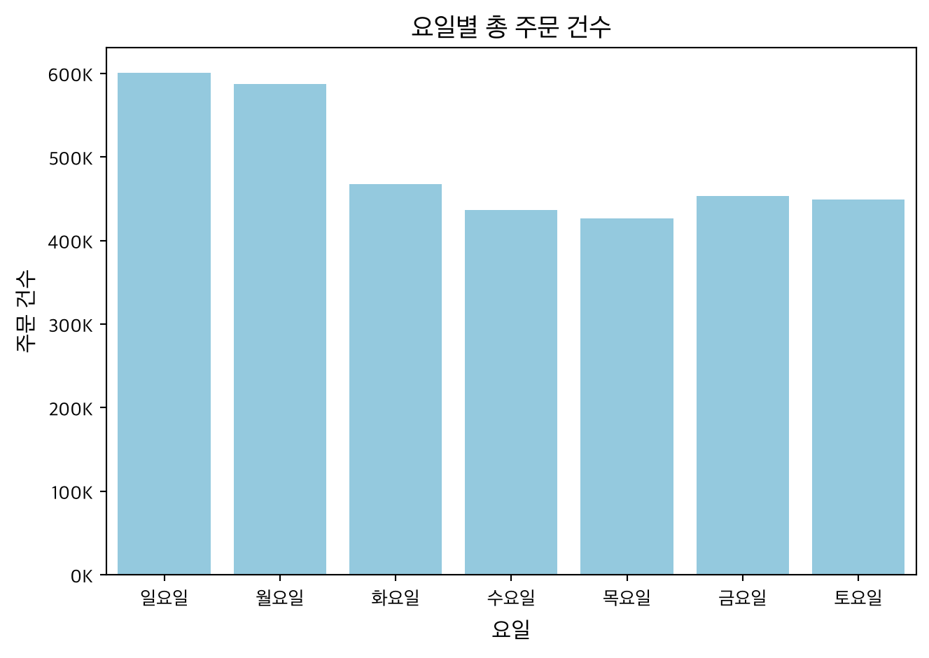
일요일(0)과 월요일(1)에 가장 많은 주문(약 60만 건 이상)이 발생하고, 주중(수~목)에는 상대적으로 주문 건수가 감소하는 명확한 주말 및 주초 집중 패턴을 시각적으로 뚜렷하게 확인할 수 있습니다.
5.3.2 가장 인기 있는 TOP 10 상품 및 카테고리 분석
PyArrow Dataset으로 스캔한 주문 상품 데이터를 메타 데이터(products, aisles, departments)와 병합(merge)하여 Instacart에서 가장 높은 주문량을 기록한 상위 10개 상품을 추출합니다.
# pandas read_parquet을 사용한 선택적 컬럼 로드 (Selective Load)
df_prior = pd.read_parquet(
    data_dir / "order_products__prior.parquet",
    engine="pyarrow",
    dtype_backend="pyarrow",
    columns=[
        "product_id",
        "reordered",
        "add_to_cart_order",
    ],
)

top10_products = (
    df_prior.groupby("product_id", observed=True)
    .agg(
        total_orders=("reordered", "count"),
        reorder_rate=("reordered", "mean"),
    )
    .reset_index()
    .merge(products, on="product_id", how="inner")
    .merge(aisles, on="aisle_id", how="inner")
    .merge(departments, on="department_id", how="inner")
    .sort_values(by="total_orders", ascending=False)
    .head(10)
    .loc[
        :,
        [
            "product_name",
            "aisle",
            "department",
            "total_orders",
            "reorder_rate",
        ],
    ]
)

top10_products| product_name | aisle | department | total_orders | reorder_rate | |
|---|---|---|---|---|---|
| 24848 | Banana | fresh fruits | produce | 472565 | 0.843501 |
| 13172 | Bag of Organic Bananas | fresh fruits | produce | 379450 | 0.832555 |
| 21133 | Organic Strawberries | fresh fruits | produce | 264683 | 0.777704 |
| ... | ... | ... | ... | ... | ... |
| 16793 | Strawberries | fresh fruits | produce | 142951 | 0.698155 |
| 26204 | Limes | fresh fruits | produce | 140627 | 0.681007 |
| 27839 | Organic Whole Milk | milk | dairy eggs | 137905 | 0.830354 |
10 rows × 5 columns
결과를 가로 막대 그래프로 시각화해 보겠습니다.
fig, ax = plt.subplots()
sns.barplot(
    data=top10_products,
    y="product_name",
    x="total_orders",
    palette="viridis",
    hue="product_name",
    legend=False,
    ax=ax,
)
ax.set_title("가장 인기 있는 TOP 10 상품", fontsize=14)
ax.set_xlabel("총 주문 건수", fontsize=12)
ax.set_ylabel("상품명", fontsize=12)

ax.xaxis.set_major_formatter(
    plt.FuncFormatter(lambda x, loc: f"{int(x/1000):,}K")
)
plt.tight_layout()
plt.show()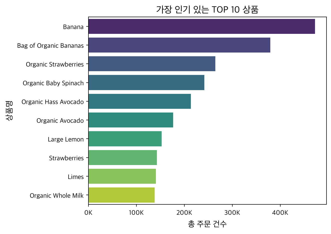
분석 결과, Banana, Bag of Organic Bananas, Organic Strawberries, Organic Baby Spinach 등 신선 식품(Produce) 부문의 품목들이 최상위를 독점하고 있으며, 재주문율(reorder_rate) 역시 75%~84%에 달할 정도로 높은 충성도를 보입니다.
5.3.3 장바구니 담는 순서와 재주문율의 관계
고객이 장바구니에 가장 먼저 담는 상품(1순위)과 나중에 담는 상품(10순위) 간의 재주문율 차이가 존재할까요?
| add_to_cart_order | total_items | reorder_rate | |
|---|---|---|---|
| 0 | 1 | 3214874 | 0.677533 |
| 1 | 2 | 3058126 | 0.676251 |
| 2 | 3 | 2871133 | 0.658037 |
| ... | ... | ... | ... |
| 7 | 8 | 1766014 | 0.573247 |
| 8 | 9 | 1562640 | 0.561474 |
| 9 | 10 | 1378293 | 0.551018 |
10 rows × 3 columns
순서에 따른 재주문율의 변화 추이를 선 그래프로 살펴보겠습니다.
fig, ax = plt.subplots()
sns.lineplot(
    data=cart_order_analysis,
    x="add_to_cart_order",
    y="reorder_rate",
    marker="o",
    color="coral",
    linewidth=2,
    ax=ax,
)
ax.set_title(
    "장바구니 담는 순서에 따른 재주문율", fontsize=14
)
ax.set_xlabel("장바구니 담는 순서", fontsize=12)
ax.set_ylabel("재주문율", fontsize=12)
ax.set_xticks(range(1, 11))
ax.set_ylim(0.5, 0.7)

# 백분율 포맷팅
ax.yaxis.set_major_formatter(
    plt.FuncFormatter(lambda x, loc: f"{x:.0%}")
)
plt.grid(True, linestyle="--", alpha=0.6)
plt.tight_layout()
plt.show()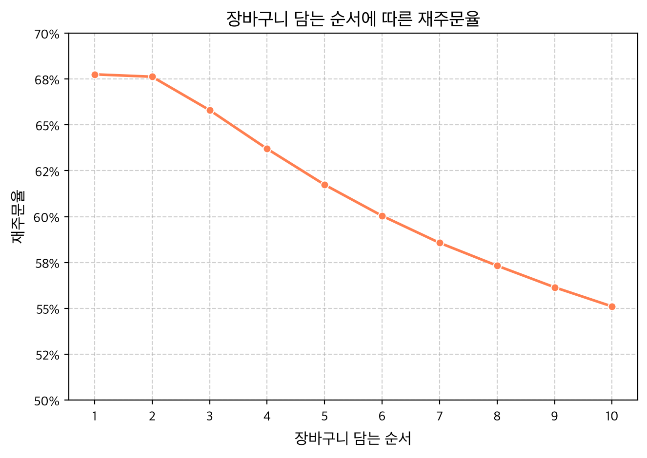
시각화에서 뚜렷하게 나타나듯, 장바구니에 1번째로 담긴 상품의 재주문율은 약 67.8%인 반면, 10번째로 담긴 상품의 재주문율은 약 55.1%로 지속적으로 감소합니다. 이는 소비자가 평소 자주 습관적으로 구매하는 생필품을 장바구니에 가장 먼저 담는 경향이 있음을 시사합니다.
5.4 to_batches()를 활용한 대용량 스트리밍 집계
pandas의 read_parquet() 함수는 기본적으로 전체 데이터를 한 번에 메모리로 로드합니다. 데이터가 시스템의 메모리(RAM) 용량을 초과할 경우, OOM(out of memory) 에러가 발생합니다.
이러한 한계를 극복하기 위해, PyArrow 백엔드의 Dataset과 to_batches()를 활용하여 전체 데이터를 배치(Chunk) 단위로 순차적으로 받아 처리하는 스트리밍(Streaming) 패턴을 구성할 수 있습니다. 이 방법을 통해 수십~수백 GB 단위의 초대용량 데이터셋도 일정한 소량의 메모리(수 MB)만 사용하여 집계를 완수할 수 있습니다.
# 상품 ID -> 부서 ID 매핑 딕셔너리 생성
prod_to_dept = dict(
    zip(
        products["product_id"].to_numpy(),
        products["department_id"].to_numpy(),
    )
)

# 스트리밍을 위한 PyArrow Dataset 준비
prior_ds = ds.dataset(
    data_dir / "order_products__prior.parquet",
    format="parquet",
)
scanner_stream = prior_ds.scanner(
    columns=["product_id", "reordered"]
)

# 누적 상태 저장 딕셔너리
dept_counts = {}
dept_reorders = {}

# 배치(Batch) 단위 스트리밍 반복문
for batch in scanner_stream.to_batches():
    tbl_batch = pa.Table.from_batches([batch])
    df_batch = tbl_batch.to_pandas()
    df_batch["department_id"] = df_batch["product_id"].map(
        prod_to_dept
    )

    grp = df_batch.groupby("department_id", observed=True)[
        "reordered"
    ].agg(["count", "sum"])

    for dept_id, row in grp.iterrows():
        if pd.isna(dept_id):
            continue
        d_id = int(dept_id)
        dept_counts[d_id] = dept_counts.get(d_id, 0) + int(
            row["count"]
        )
        dept_reorders[d_id] = dept_reorders.get(
            d_id, 0
        ) + int(row["sum"])

# 최종 누적 결과를 데이터프레임으로 변환
dept_summary = (
    pd.DataFrame(
        {
            "department_id": list(dept_counts.keys()),
            "total_orders": list(dept_counts.values()),
            "reorder_sum": list(dept_reorders.values()),
        }
    )
    .assign(
        reorder_rate=lambda df: df["reorder_sum"]
        / df["total_orders"]
    )
    .merge(departments, on="department_id", how="inner")
    .sort_values(by="total_orders", ascending=False)
    .loc[:, ["department", "total_orders", "reorder_rate"]]
)

dept_summary| department | total_orders | reorder_rate | |
|---|---|---|---|
| 3 | produce | 9479291 | 0.649913 |
| 15 | dairy eggs | 5414016 | 0.669969 |
| 18 | snacks | 2887550 | 0.574180 |
| ... | ... | ... | ... |
| 20 | missing | 69145 | 0.395849 |
| 1 | other | 36291 | 0.407980 |
| 9 | bulk | 34573 | 0.577040 |
21 rows × 3 columns
부서별 총 주문 건수를 시각화하여 확인해 보겠습니다.
fig, ax = plt.subplots()
sns.barplot(
    data=dept_summary.head(10),
    y="department",
    x="total_orders",
    palette="magma",
    hue="department",
    legend=False,
    ax=ax,
)
ax.set_title(
    "부서(Department)별 총 주문 건수 TOP 10", fontsize=14
)
ax.set_xlabel("총 주문 건수", fontsize=12)
ax.set_ylabel("부서명", fontsize=12)

ax.xaxis.set_major_formatter(
    plt.FuncFormatter(lambda x, loc: f"{int(x/1000000):,}M")
)
plt.tight_layout()
plt.show()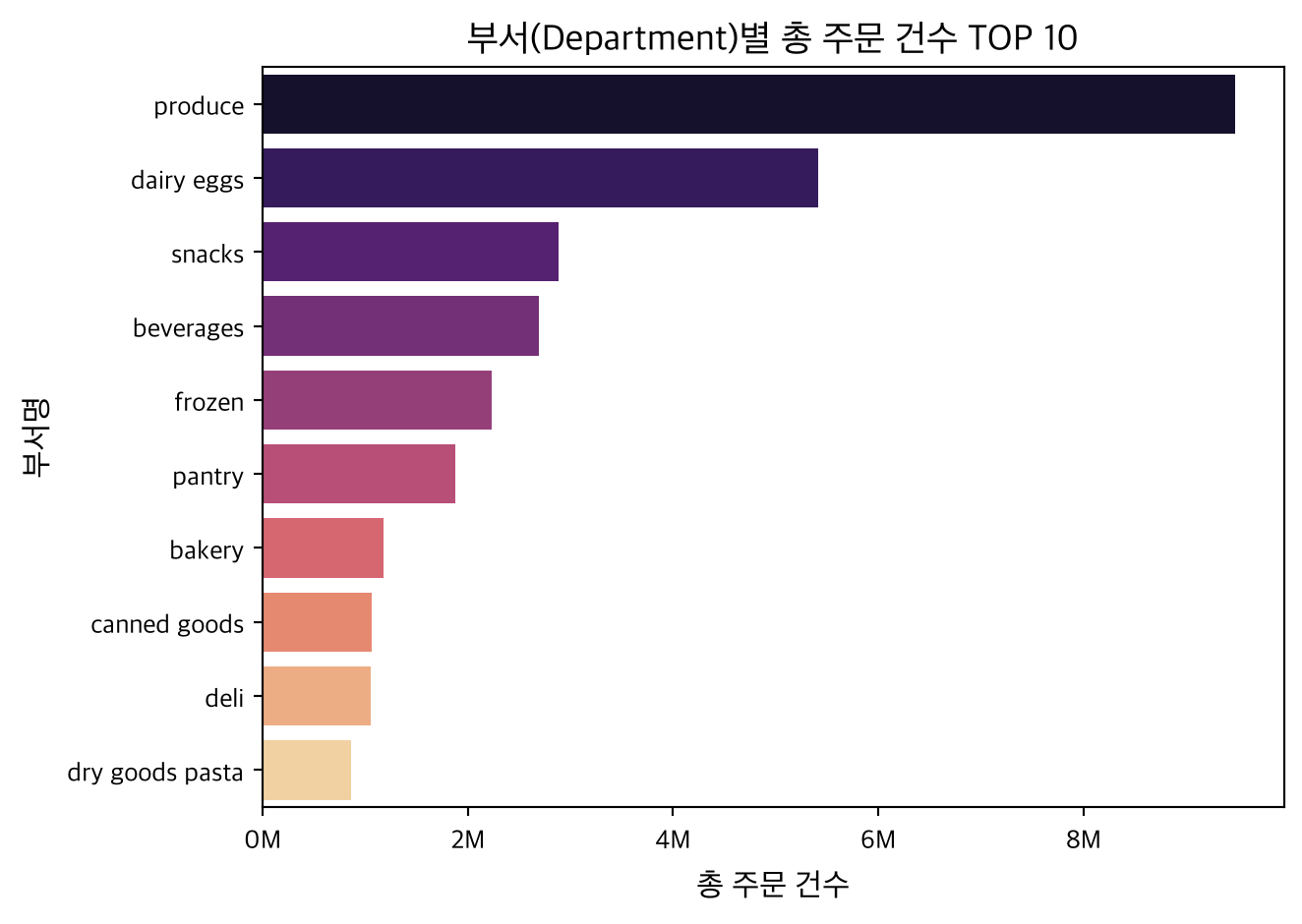
그림 5.4를 보면 produce와 dairy eggs 부서가 전체 장바구니 주문의 압도적인 비중을 차지하고 있음을 알 수 있습니다. 반면, pantry나 dry goods pasta와 같은 장기 보관 식품은 상대적으로 낮은 재주문율(34%~46%)을 나타냅니다.